Branch-Line Coupler | Yaniv Lieberman

Initial HFSS branch-line coupler implementation over FR-4

July 8, 2026

Project Sections

Introduction
Branch-line coupler theory
Design goals and specifications
Ideal ADS simulation
Branch length and bandwidth sweep
Microstrip implementation
Layout implementation and HFSS EM simulation
Comparison and discussion
Summary and engineering takeaways

1. Introduction

A branch-line coupler is a four-port microwave network that divides an input signal equally between two output ports while maintaining a 90° phase difference between them. Ideally, the fourth port is isolated and receives no power from the excited input.

This project develops a microstrip 90° hybrid coupler from initial circuit synthesis through full-wave electromagnetic validation. The design begins with an ideal transmission-line model in Keysight ADS, where the required quarter-wave impedances and electrical lengths are established. The electrical design is then converted into a physical microstrip layout and evaluated in Ansys HFSS.

The goal of the project is not only to verify the nominal 3 GHz design, but also to examine how branch dimensions influence center frequency, amplitude balance, phase imbalance, and usable bandwidth.

2. Branch-Line Coupler Theory

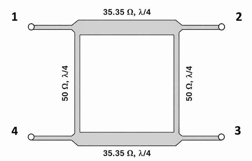
A branch-line coupler is formed by four quarter-wavelength transmission-line sections arranged as a square. When Port 1 is excited, Ports 2 and 3 are the useful outputs, while Port 4 is the isolated port.

**Figure 1:** Equal-split branch-line coupler topology and port numbering.

Quarter-wave operation

Each branch is designed to be electrically 90° long at the center frequency:

\[\theta = \beta l = 90^\circ\]

For a microstrip implementation, the initial physical length is approximately one quarter of the guided wavelength:

\[l \approx \frac{\lambda_g}{4}=\frac{c}{4f_0\sqrt{\varepsilon_\text{eff}}}\]

Because \(\varepsilon_\text{eff}\) depends on trace width and substrate geometry, the final lengths are synthesized in ADS LineCalc and then refined through HFSS simulation.

Equal-split impedance synthesis

For a conventional equal-split branch-line coupler with system impedance \(Z_0\), the horizontal branches use \(Z_0/\sqrt{2}\) and the vertical branches use \(Z_0\):

\[Z_\text{horizontal}=\frac{Z_0}{\sqrt{2}}, \qquad Z_\text{vertical}=Z_0\]

For a 50 Ω system, this gives 35.35 Ω horizontal branches and 50 Ω vertical branches. The 35.35 Ω branches control the equal power division, while the 50 Ω branches complete the phase relationships required for matching and isolation.

Ideal scattering behavior

At the design frequency, the ideal equal-split response is:

\[|S_{21}|=|S_{31}|=\frac{1}{\sqrt{2}} \approx -3.01\ \text{dB}\]

The input should be matched, the isolated port should receive negligible power, and the two output paths should remain in quadrature:

\[S_{11}\approx0,\qquad S_{41}\approx0,\qquad \angle\left(\frac{S_{21}}{S_{31}}\right)\approx90^\circ\]

The branch-line coupler is inherently narrowband because the match, isolation, and phase conditions depend on all four branches remaining close to 90° electrical length.

3. Design Goals and Specifications

The objective was to design a 3 GHz equal-split branch-line hybrid coupler for a 50 Ω microwave system. The physical implementation uses the same generic FR-4 stackup used in the earlier microstrip and Wilkinson-divider projects.

Parameter	Design target
Center frequency	3 GHz
Reference impedance	50 Ω
Coupling ratio	Equal split
Output magnitude	Approximately -3 dB at Ports 2 and 3
Output phase difference	90°
Input return loss	Better than -20 dB near 3 GHz
Port 1 to Port 4 isolation	Better than -20 dB near 3 GHz
Implementation	Microstrip on FR-4
Substrate parameters	\(\varepsilon_r=4.3\), \(h=1.6\ \text{mm}\), \(t=35\ \mu\text{m}\)

Amplitude balance was evaluated as the magnitude difference between the two output paths:

\[\Delta A = \left|\text{dB}(S_{31})-\text{dB}(S_{21})\right|\]

Phase balance was evaluated relative to the ideal quadrature condition:

\[\Delta \phi = \left|\angle\left(\frac{S_{21}}{S_{31}}\right)-90^\circ\right|\]

4. Ideal ADS Simulation

The branch-line coupler was first verified in ADS using an ideal TLIN model. This establishes the expected behavior before microstrip effects such as junction discontinuities, conductor loss, dielectric loss, and radiation are included.

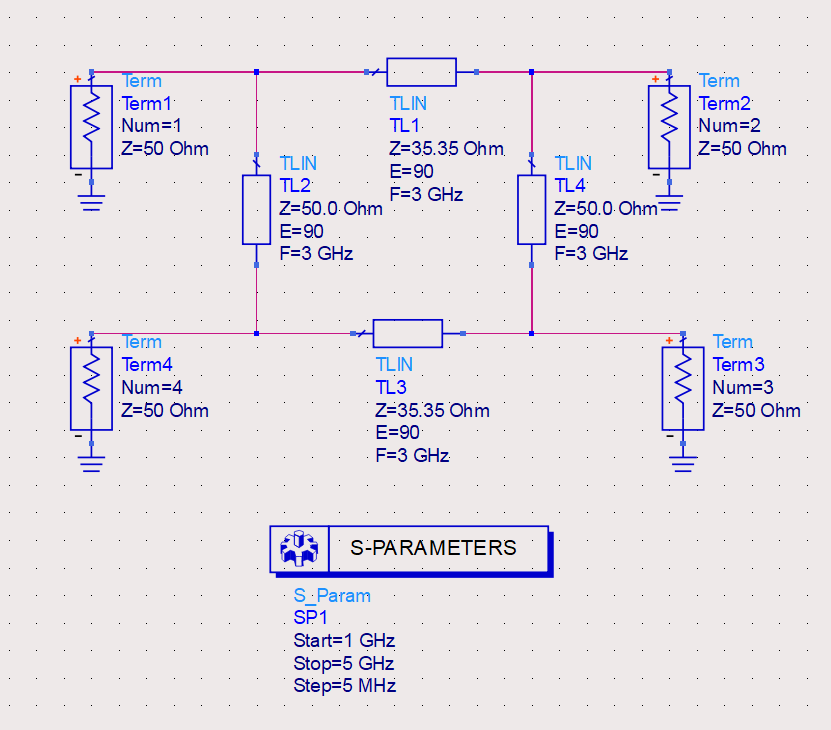
Ideal ADS branch-line coupler schematic — **Figure 2:** Ideal ADS transmission-line model and S-parameter simulation setup.

The top and bottom branches were assigned 35.35 Ω, while the left and right branches were assigned 50 Ω. All four lines were set to 90° electrical length at the 3 GHz design frequency and simulated from 1 GHz to 5 GHz.

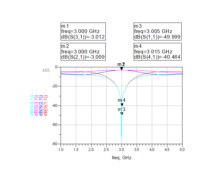
**Figure 3:** Ideal S-parameter response of the branch-line coupler.

At 3 GHz, the ideal model produced \(S_{21}=-3.009\ \text{dB}\) and \(S_{31}=-3.012\ \text{dB}\), essentially the expected lossless -3.01 dB equal split. The input match and isolation also showed deep nulls near 3 GHz, with \(S_{11}\) around -50 dB and \(S_{41}\) around -40.5 dB.

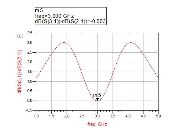
Ideal output amplitude difference — **Figure 4:** Output amplitude difference between the coupled and through paths.

The output amplitude difference at 3 GHz was only -0.003 dB, confirming that the two output ports receive nearly identical power at the center frequency.

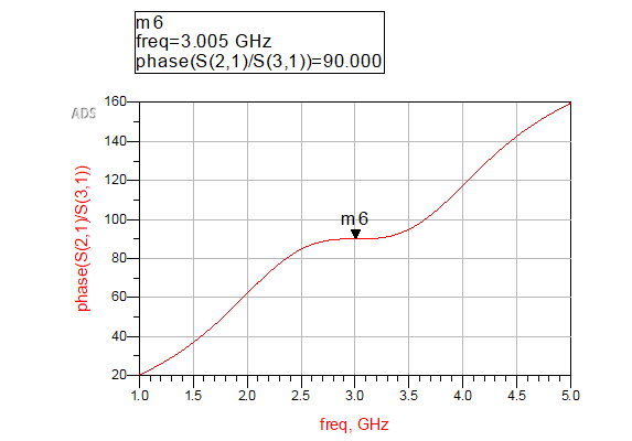
Ideal output phase difference — **Figure 5:** Phase difference between the through and coupled output paths.

The phase of \(S_{21}/S_{31}\) was 90° near 3 GHz, confirming the expected quadrature relationship between the two equal-amplitude output signals.

Metric	Ideal ADS result
\(S_{21}\) at 3 GHz	-3.009 dB
\(S_{31}\) at 3 GHz	-3.012 dB
Output amplitude difference	-0.003 dB
Output phase difference	90°
\(S_{11}\), near 3 GHz	about -50 dB
\(S_{41}\), near 3 GHz	about -40.5 dB

5. Branch Length and Bandwidth Sweep

Because the coupler depends on four quarter-wave sections, the useful operating band is limited by how closely the branches remain near 90° electrical length. The ideal ADS model was evaluated with three requirements: \(S_{11},S_{41}\le -20\ \text{dB}\), amplitude imbalance within 0.5 dB, and phase difference within \(90^\circ\pm5^\circ\).

Nominal bandwidth

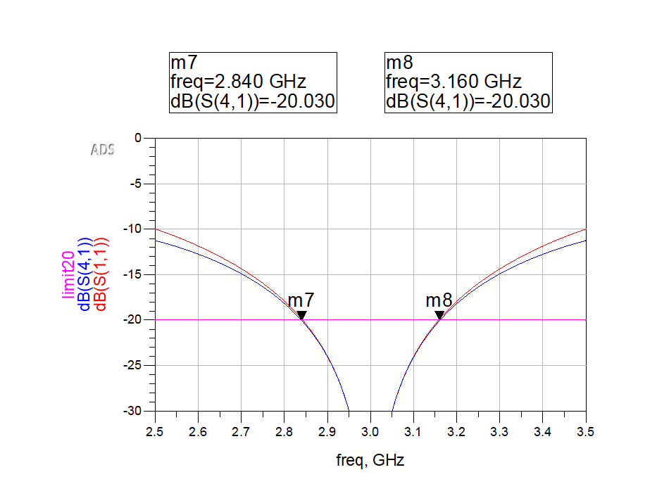
Ideal input return loss and isolation bandwidth — **Figure 6:** Ideal input return loss and isolation near the 3 GHz design frequency, with the -20 dB performance threshold.

The match and isolation response was the limiting criterion in the ideal model. The isolation response crossed the -20 dB threshold near 2.84 GHz and 3.16 GHz.

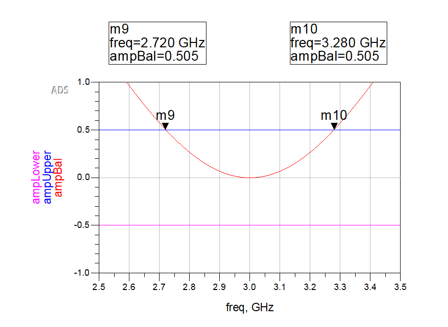
Ideal output amplitude balance bandwidth — **Figure 7:** Output amplitude balance of the ideal branch-line coupler. The +/-0.5 dB limits are satisfied over a wider range than the match/isolation requirement.

Ideal output phase difference bandwidth — **Figure 8:** Output phase difference between Ports 2 and 3. The phase remains within 90 degrees +/-5 degrees over a broad range around the design frequency.

Requirement	Approximate valid range
Isolation, \(S_{41}\le -20\ \text{dB}\)	2.84-3.16 GHz
Amplitude imbalance within 0.5 dB	2.72-3.28 GHz
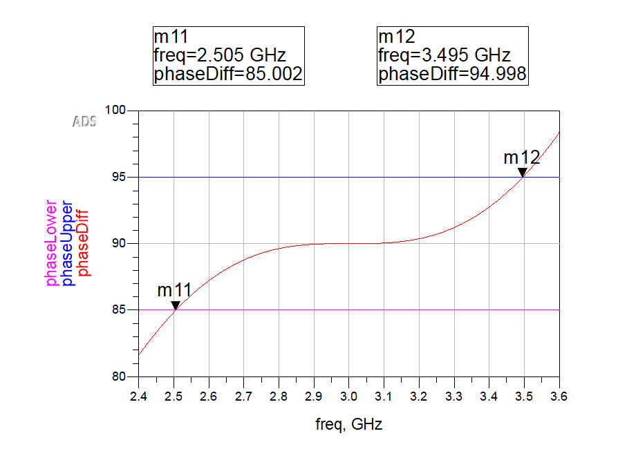
Phase difference within \(90^\circ\pm5^\circ\)	2.505-3.495 GHz

\[BW_\text{ideal} = 3.16-2.84 = 0.32\ \text{GHz} = 320\ \text{MHz}\]

\[FBW_\text{ideal}=\frac{3.16-2.84}{3.00}\times100\%\approx10.7\%\]

Common branch-length sweep

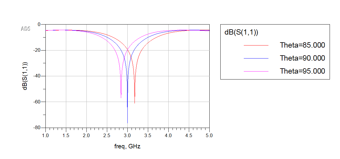
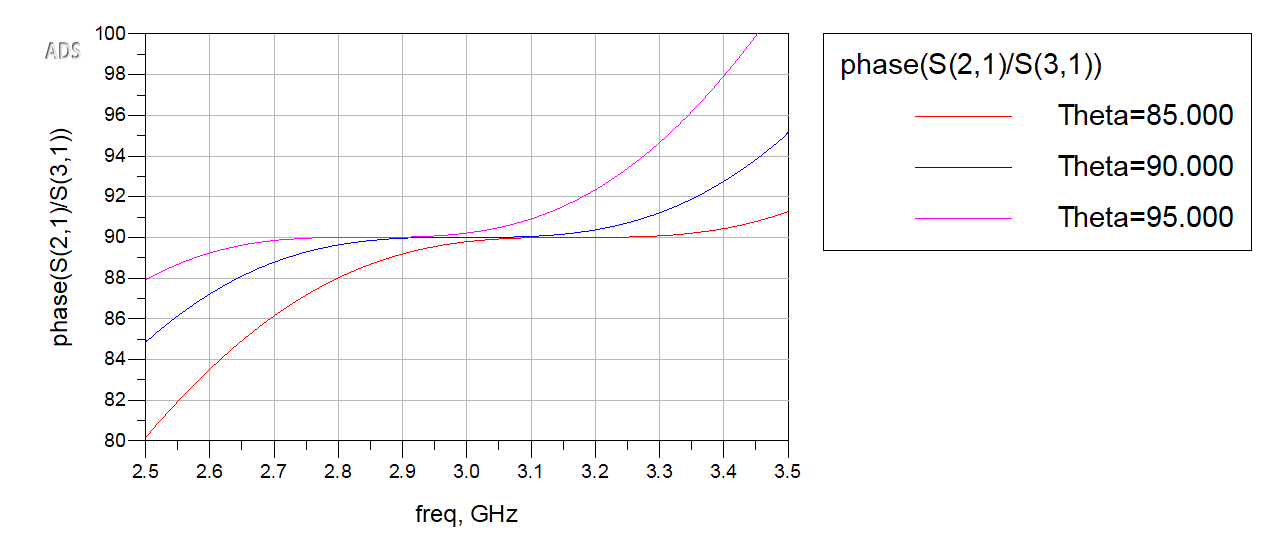
A common electrical-length sweep was then performed by setting all four ideal branches to 85°, 90°, and 95° at the 3 GHz reference frequency.

Common branch length sweep phase difference — **Figure 10:** Effect of common branch electrical length on output phase difference. The quadrature condition shifts with the return-loss minimum.

Electrical length at 3 GHz	Relative branch length	Approximate shifted center frequency
85°	Shorter than nominal	3.18 GHz
90°	Nominal	3.00 GHz
95°	Longer than nominal	2.84 GHz

Changing all four branches by the same amount primarily translates the ideal response in frequency. In a physical microstrip implementation, the shift is not perfectly self-similar because dispersion, finite-width effects, loss, junctions, and ports also influence the response.

6. Microstrip Implementation

The ideal transmission-line model was then converted into an ADS MLIN distributed microstrip implementation. This model retains the branch impedances and quarter-wave design intent while adding substrate-dependent propagation, conductor loss, and dielectric loss.

Branch type	Target impedance	Width	Electrical length	Initial physical length
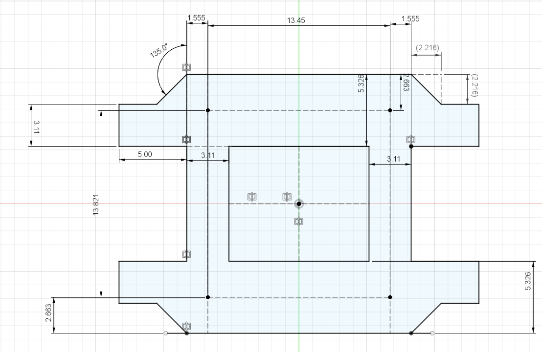
Horizontal branches	35.35 Ω	5.326 mm	90° at 3 GHz	13.450 mm
Vertical branches	50 Ω	3.110 mm	90° at 3 GHz	13.821 mm

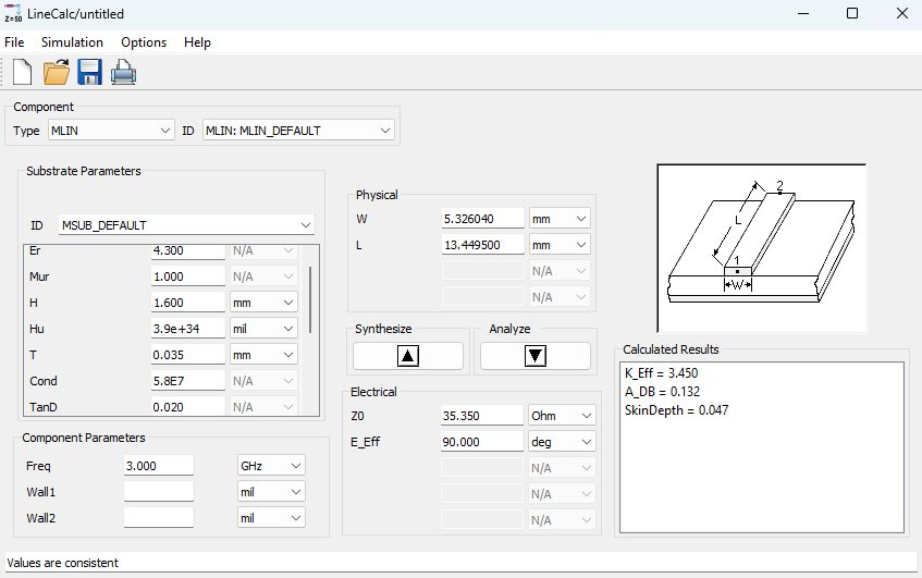
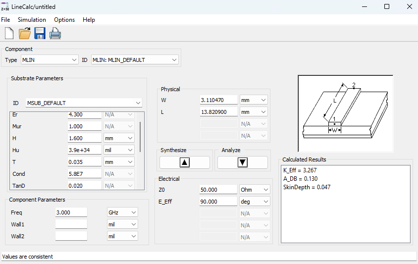
ADS LineCalc 35.35 ohm branch — **Figure 11:** ADS LineCalc synthesis of the 35.35 Ω horizontal microstrip branch.

ADS LineCalc 50 ohm branch — **Figure 12:** ADS LineCalc synthesis of the 50 Ω vertical microstrip branch.

The lower-impedance horizontal lines require a wider trace. Their larger width produces a slightly higher effective dielectric constant than the 50 Ω lines, so their physical quarter-wave length is slightly shorter.

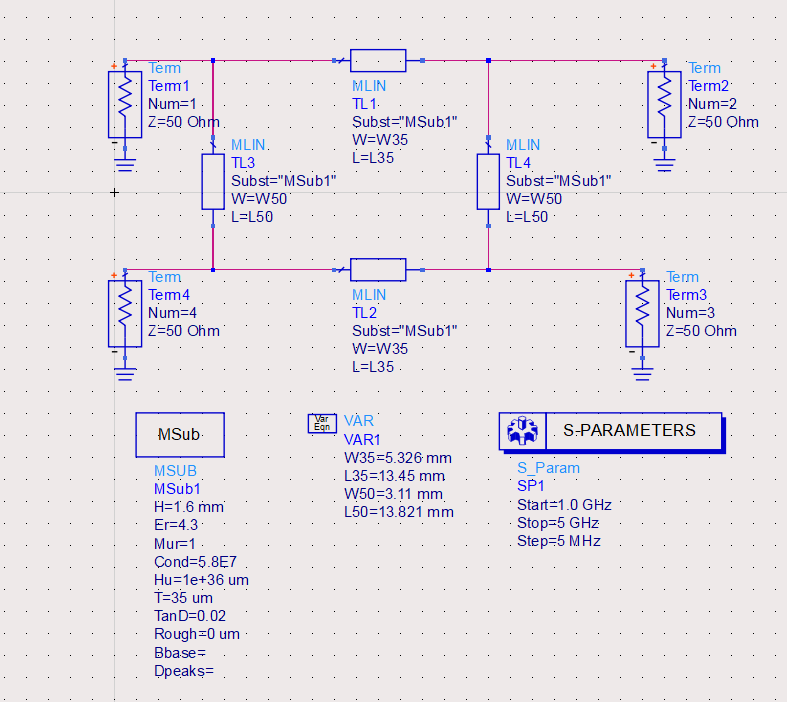
ADS MLIN branch-line coupler schematic — **Figure 13:** ADS distributed microstrip (MLIN) implementation of the branch-line coupler.

The MLIN model remains a schematic-level microstrip model: it captures line loss and propagation, but it still connects branch endpoints as ideal schematic nodes. It does not yet model finite-width T-junction discontinuities, which are included later in HFSS.

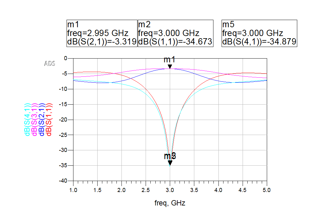
ADS MLIN S-parameter results — **Figure 14:** Simulated MLIN S-parameters showing approximately equal output splitting, low input reflection, and low isolation-port power near 3 GHz.

The MLIN response stayed centered very close to 3 GHz. The through-path response reached approximately -3.319 dB near 2.995 GHz, about 0.31 dB below the lossless ideal value because of conductor and dielectric loss in the FR-4 microstrip model.

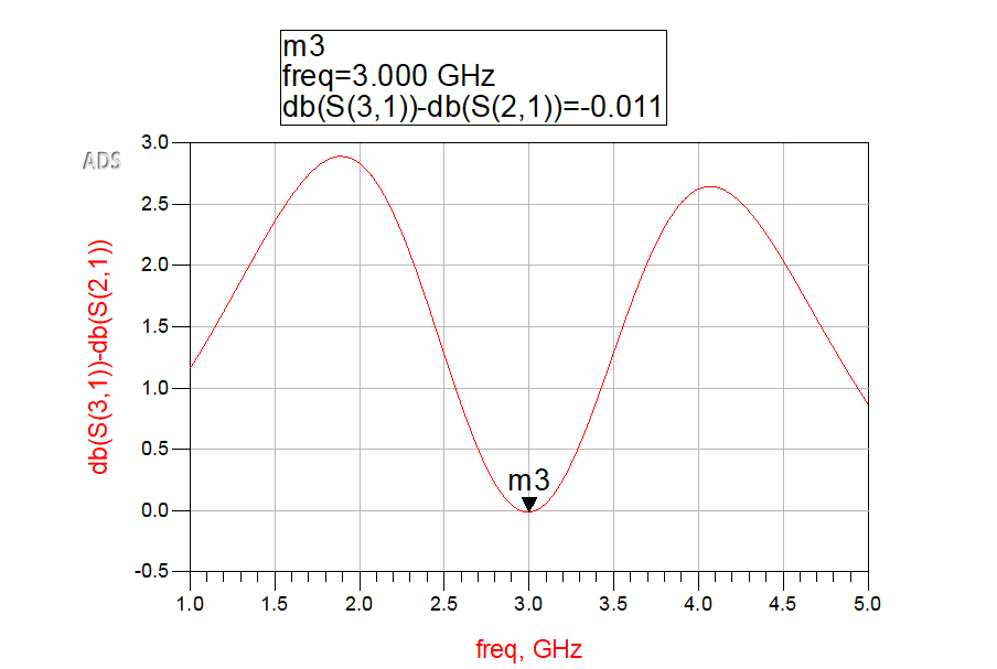
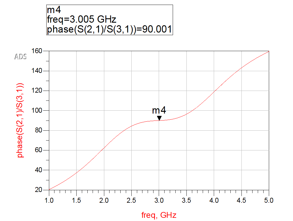
ADS MLIN output amplitude balance — **Figure 15:** Output amplitude balance of the ADS MLIN implementation.

ADS MLIN output phase difference — **Figure 16:** Output phase difference of the ADS MLIN implementation.

At 3 GHz, the MLIN model gave \(S_{11}=-34.673\ \text{dB}\), \(S_{41}=-34.879\ \text{dB}\), amplitude difference of -0.011 dB, and phase difference of 90.001° at the nearest simulated point.

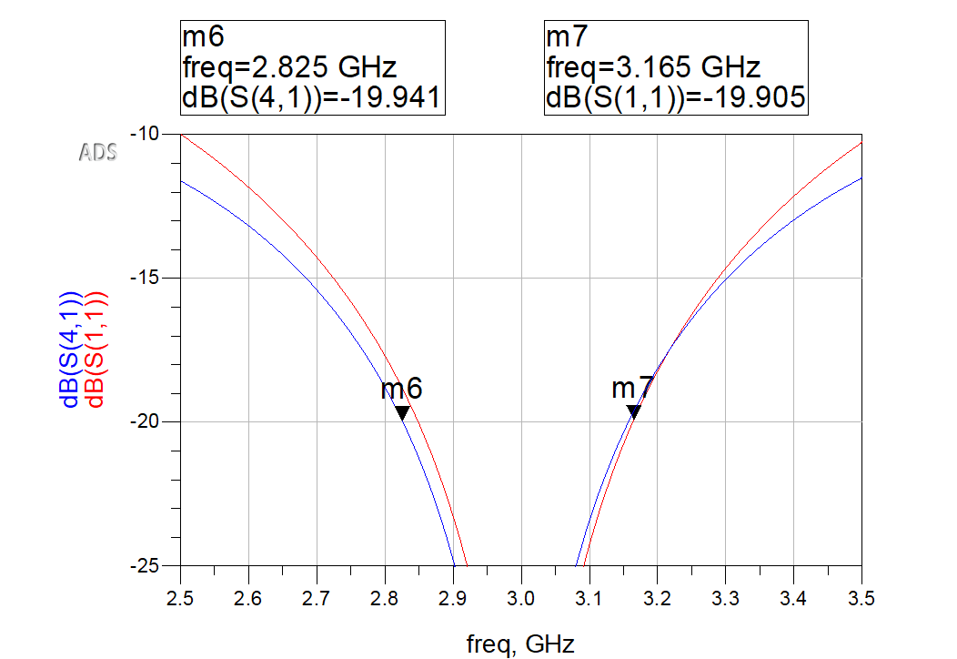
ADS MLIN match and isolation bandwidth — **Figure 17:** ADS MLIN input return loss and isolation near the design frequency. The -20 dB crossings indicate an approximately 2.825-3.165 GHz match/isolation bandwidth.

The MLIN match/isolation bandwidth was approximately 2.825-3.165 GHz, or about 340 MHz. This is slightly wider than the ideal model's 320 MHz match/isolation bandwidth, although the complete usable-bandwidth definition should also include amplitude and phase balance.

7. Layout Implementation and HFSS EM Simulation

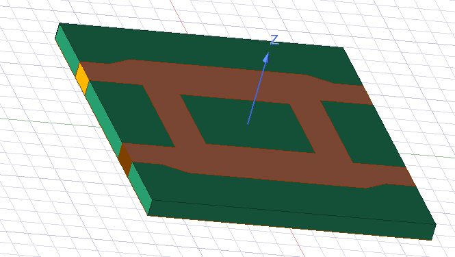
After the ADS ideal and MLIN stages, the coupler was implemented in HFSS for full-wave electromagnetic simulation. The HFSS model evaluates the actual three-dimensional structure, including finite trace width, junction effects, port discontinuities, substrate behavior, and electromagnetic coupling between branches.

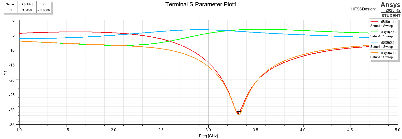
**Figure 18:** Physical branch-line coupler layout sketch created from the ADS LineCalc dimensions. The 35.35 Ω branches use wider traces, while the 50 Ω branches and feed lines use narrower traces.

Initial HFSS branch-line coupler model — **Figure 19:** Initial HFSS implementation using the ADS-derived microstrip dimensions over FR-4 with a continuous ground plane and four lumped terminal ports.

The first HFSS simulation showed that the response shifted above the intended 3 GHz design frequency. The main matching/isolation null appeared near 3.315 GHz, indicating that the physical HFSS layout was electrically shorter than the ideal and MLIN ADS models.

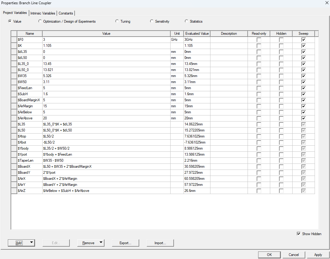
Initial HFSS S-parameter response before tuning — **Figure 20:** Initial HFSS S-parameter response before length tuning. The response is centered near 3.315 GHz instead of 3 GHz, indicating that the physical HFSS layout is electrically shorter than the design target.

To correct the shift, a common length-scaling factor was applied:

\[K=\frac{f_\text{HFSS}}{f_0}=\frac{3.315}{3.000}=1.105\]

The branch lengths were then scaled from the original LineCalc values:

\[L_{35}=K L_{35,0}=14.862\ \text{mm}, \qquad L_{50}=K L_{50,0}=15.272\ \text{mm}\]

HFSS project variables for parametric model — **Figure 21:** HFSS project variables used for the parametric branch-line coupler model. The main tuning factor was set to K = 1.105, giving tuned branch lengths of L35 = 14.862 mm and L50 = 15.272 mm.

The tuned HFSS response is shown below. At 3 GHz, the input match and isolation were both strong, and the output ports showed the expected split behavior.

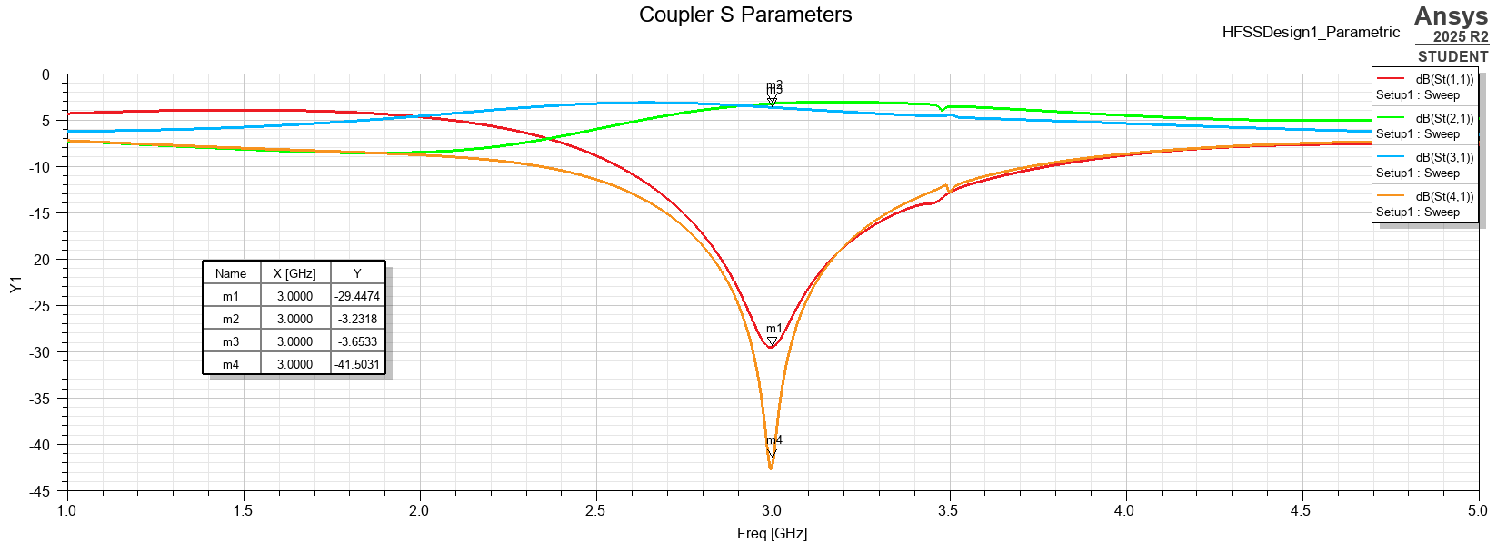
**Figure 22:** Tuned HFSS S-parameter response of the parametric branch-line coupler. At 3 GHz, the model shows strong input matching and isolation with S11 ≈ -29.45 dB and S41 ≈ -41.50 dB.

Quantity	HFSS result at 3 GHz
\(S_{11}\)	-29.45 dB
\(S_{21}\)	-3.23 dB
\(S_{31}\)	-3.65 dB
\(S_{41}\)	-41.50 dB

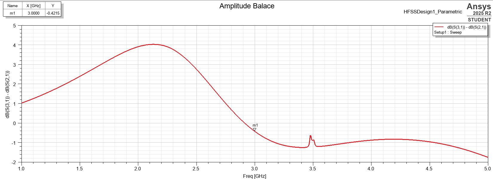
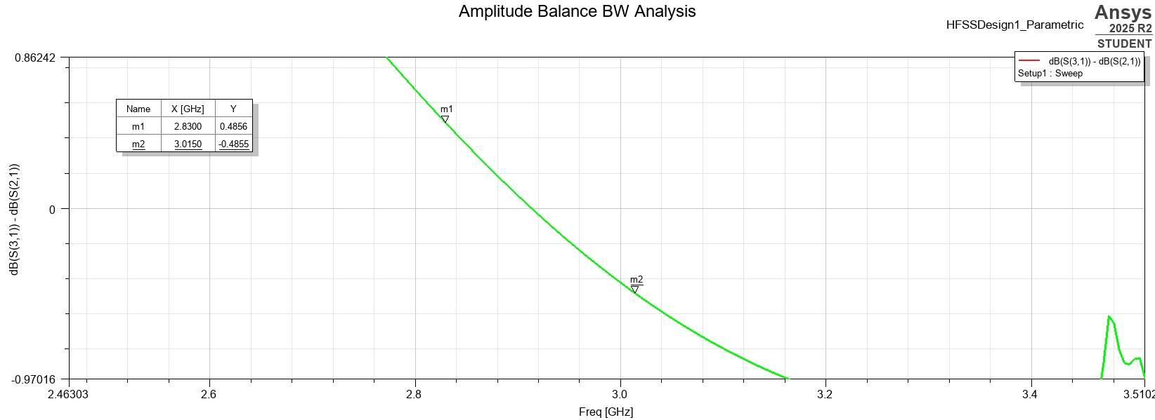
**Figure 23:** Tuned HFSS output amplitude balance calculated as dB(S31)-dB(S21). At 3 GHz, the amplitude imbalance is approximately -0.42 dB.

At 3 GHz, the amplitude imbalance was \(\Delta A=-0.4215\ \text{dB}\), which satisfies the selected ±0.5 dB criterion, although it is close to the upper-frequency edge of the valid amplitude-balance range.

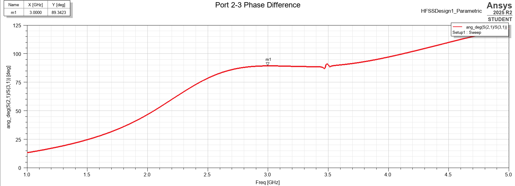
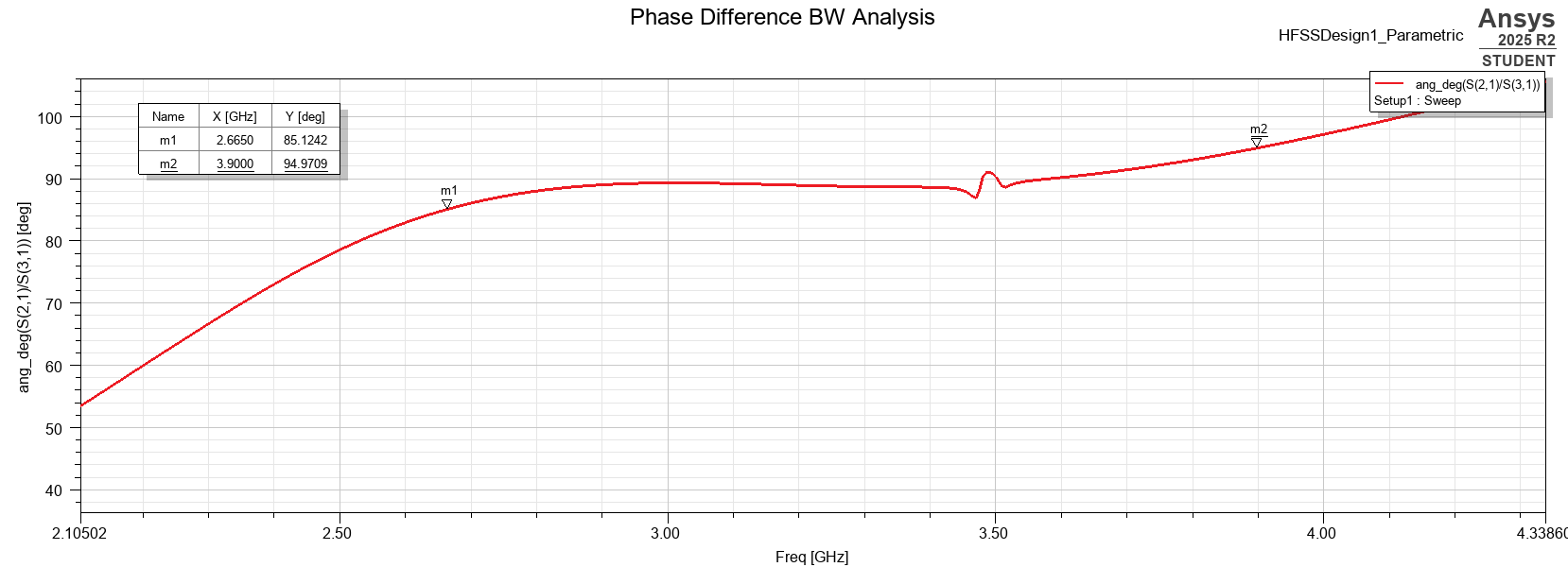
Tuned HFSS output phase difference — **Figure 24:** Tuned HFSS phase difference between the output ports, calculated as ∠(S21/S31). At 3 GHz, the phase difference is approximately 89.34 degrees.

The output phase difference at 3 GHz was 89.34°, very close to the ideal quadrature condition.

HFSS usable bandwidth

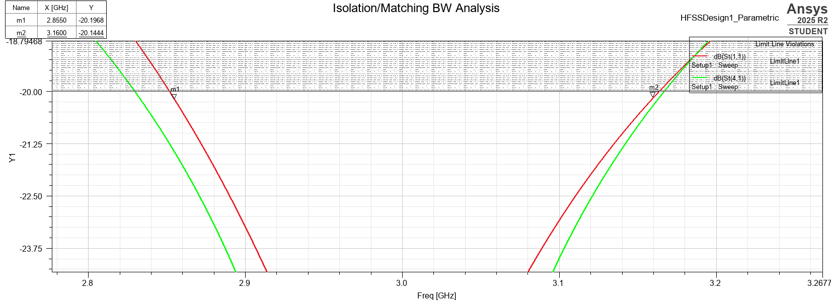
The same bandwidth criteria used for the ideal ADS model were applied to the tuned HFSS result:

\[S_{11},S_{41}\le -20\ \text{dB}, \quad |\text{dB}(S_{31})-\text{dB}(S_{21})|\le0.5\ \text{dB}, \quad 85^\circ\le\angle(S_{21}/S_{31})\le95^\circ\]

HFSS match and isolation bandwidth — **Figure 25:** HFSS input matching and isolation bandwidth analysis. Using the -20 dB criterion, the valid range is approximately 2.855 GHz to 3.160 GHz.

HFSS amplitude balance bandwidth — **Figure 26:** HFSS amplitude-balance bandwidth analysis using the +/-0.5 dB criterion. The amplitude balance is valid from approximately 2.830 GHz to 3.015 GHz.

HFSS phase bandwidth — **Figure 27:** HFSS phase-difference bandwidth analysis using the 90 degrees +/-5 degrees criterion. The phase criterion is satisfied from approximately 2.665 GHz to 3.900 GHz.

Criterion	Limit	Valid HFSS range
Input match / isolation	\(S_{11},S_{41}\le -20\ \text{dB}\)	2.855-3.160 GHz
Amplitude balance	\(\|\Delta A\|\le0.5\ \text{dB}\)	2.830-3.015 GHz
Phase balance	\(90^\circ\pm5^\circ\)	2.665-3.900 GHz
Final usable bandwidth	All criteria satisfied	2.855-3.015 GHz

\[BW_\text{HFSS}=3.015-2.855=0.160\ \text{GHz}=160\ \text{MHz}\]

\[FBW_\text{HFSS}=\frac{160\ \text{MHz}}{3\ \text{GHz}}\times100\%\approx5.3\%\]

The final HFSS bandwidth was limited mainly by output amplitude imbalance. Phase balance remained valid over a much wider range, and match/isolation remained valid to a higher upper frequency than the final usable band.

8. Comparison and Discussion

The coupler was evaluated using three modeling levels: an ideal ADS TLIN model, an ADS MLIN distributed microstrip model, and a full-wave HFSS EM model. Each stage added more physical detail and therefore produced a more realistic result.

Model	Center-frequency behavior	Comment
Ideal ADS TLIN	3.0 GHz	Theoretical lossless quarter-wave response
ADS MLIN	Near 3.0 GHz	Physical microstrip with loss and dispersion
Initial HFSS	About 3.315 GHz	Full-wave layout electrically too short
Tuned HFSS	Near 3.0 GHz	Corrected using branch-length scaling

Metric	Ideal ADS	ADS MLIN	Tuned HFSS
\(S_{21}\)	-3.009 dB	-3.319 dB	-3.23 dB
\(S_{31}\)	-3.012 dB	about -3.33 dB	-3.65 dB
\(S_{11}\)	about -50 dB	-34.67 dB	-29.45 dB
\(S_{41}\)	about -40.5 dB	-34.88 dB	-41.50 dB
Amplitude imbalance	-0.003 dB	-0.011 dB	-0.4215 dB
Phase difference	90.0°	90.001°	89.34°

Model	Final usable bandwidth	Fractional bandwidth	Main limiting factor
Ideal ADS	2.84-3.16 GHz	about 10.7%	Isolation
Tuned HFSS	2.855-3.015 GHz	about 5.3%	Amplitude imbalance

The comparison shows why full-wave validation is important for microwave layout design. The ideal model verified the topology, and the MLIN model provided a first physical microstrip approximation. HFSS then revealed layout-level effects from finite-width junctions, feed transitions, substrate/ground behavior, and port discontinuities.

The initial HFSS upward frequency shift was the key practical result. It showed that even when microstrip lengths are correct according to LineCalc, the complete physical layout can behave differently because the coupler is not just four isolated transmission lines. The junctions and feed regions are part of the electromagnetic structure.

9. Summary and Engineering Takeaways

This project designed and validated a 3 GHz microstrip branch-line hybrid coupler using a progressive RF workflow: theoretical synthesis, ideal ADS simulation, ADS MLIN microstrip implementation, and full-wave HFSS validation.

For a 50 Ω equal-split hybrid coupler, the horizontal branches were designed as 35.35 Ω quarter-wave sections and the vertical branches as 50 Ω quarter-wave sections. The ideal ADS model verified equal power split, high isolation, good input match, and a 90° output phase difference.

The MLIN implementation introduced realistic microstrip widths, substrate height, dielectric constant, conductor loss, dielectric loss, and effective dielectric constant. The MLIN response stayed close to the ideal result, but showed the expected additional insertion loss compared with the lossless TLIN model.

The first HFSS layout shifted above the intended 3 GHz center frequency, so the design was rebuilt parametrically and tuned with the scaling factor \(K=1.105\). The final tuned HFSS model achieved strong input matching, strong isolation, acceptable amplitude balance, and near-quadrature phase difference at 3 GHz.

Metric	Final HFSS result at 3 GHz
\(S_{11}\)	-29.45 dB
\(S_{21}\)	-3.23 dB
\(S_{31}\)	-3.65 dB
\(S_{41}\)	-41.50 dB
Amplitude imbalance	-0.4215 dB
Phase difference	89.34°

The final overlapping usable bandwidth was 2.855-3.015 GHz, or 160 MHz, corresponding to approximately 5.3% fractional bandwidth. This is narrower than the ideal ADS bandwidth because the full-wave model includes realistic layout effects that are not captured by ideal schematic transmission-line models.

The main takeaway is that ideal transmission-line synthesis is a necessary starting point, but final microwave layout validation requires EM simulation. ADS establishes the theory, MLIN checks the physical transmission-line dimensions, and HFSS validates the full layout geometry.

Overall, the result is a 3 GHz branch-line coupler that performs well in full-wave simulation and clearly demonstrates the importance of EM validation when moving from schematic-level RF design to physical microwave layout.

Back to Portfolio